Results of the first part of INTENS project

The aim of INTENS was to investigate the nature of fluctuations of the magnetic field and electron density and their scaling features in different geomagnetic disturbance conditions to unveil the role played by magnetohydrodynamic (MHD) turbulence in generating multi-scale plasma structures and plasma inhomogeneities. The analysis of Swarm constellation measurements of the Earth's magnetic field as well as electron density allowed us to achieve this goal.

We will first give some information on how data have been selected and pre-treated, along with the basic description of the methods used for the analyses, and then we will show some of the most interesting results of the project.

1. Data selection and preliminary analysis.

• Swarm A and B magnetic and plasma data, at 1 Hz cadence, have been downloaded from the ESA Swarm dissemination server: ftp://swarm-diss.eo.esa.int , spanning the time period between April 1^st 2014 to March 31^th 2018.
• Magnetic data (Level 1b product type: MAGx_LR): 1) the three components of the observed geomagnetic field have been extracted, and the CHAOS-6 model (Finlay et al., 2016) has been applied in order to subtract the internal components of the field (core and crust), which are the strongest in magnitude (tens of thousands nT) but slowly varying in time, and isolate the "external" components, which show the rapid variations related to the solar wind – magnetosphere – ionosphere coupling; 2) the resulting B_ext has been transformed in a Quasi-Dipole (QD, Emmert et al, 2010) geomagnetic reference frame, and projected in direction parallel (B_∥) and perpendicular (B_o1, B_o2) to the main field, in order to be able to investigate fluctuation dynamics which are strongly field-aligned.
• Plasma data (Level 1b product type: EFIxLPI): 1) Electron density (N_e) and temperature have been extracted and data flagged as "non nominal" (parameters  Flags_Ne and Flags_Te different from either 10 or 20, following the recommendations in the "Swarm Level 1b Product Definition" document) have been excluded; 2) A detailed analysis on the electron temperature anomalies has been performed, leading to conclude that such parameter cannot be used for the kind of analyses done in the framework of INTENS, because of the high number of gaps/invalid values and the massive occurrence of bursts of very high values whose origin is still under investigation.
• Other supplementary datasets: for supporting the analyses, and further selections on data, the following datasets have been taken into account: 1) geomagnetic indices AE and SIM-H at 1 minute cadence; 2) Interplanetary magnetic field and solar wind density and velocity at 1 minute cadence. The source of these datasets is the OMNI database.

2. Nonlinear and scaling analysis methods

2.1 Scaling features analysis

Many natural systems in stationary and/or non-equilibrium states display large fluctuations occurring over a wide range of spatial and temporal scales. This is for instance the case of space plasma systems in a turbulent regime. Turbulence is indeed a peculiar physical phenomenon occurring in non-equilibrium fluid systems characterised by occurrence of a mess of multiscale fluctuations over a very wide range of spatial and temporal scales. This mess of fluctuations are due to a continuous transfer of energy from the injection scales to the dissipation ones.

In spite of the wide range of spatio-temporal scales where fluctuations are present, according to the general picture of the Richardson's cascade, turbulent media develop a special interval of spatial and temporal scales where the mess of excited scale are characterized by a special kind of symmetry features, namely scale invariance. The manifestation of scale invariance in a fluctuation field implies the absence of a characteristic length or timescale for the emerging fluctuation structures, i.e., the occurrence of self-similarity in a statistical sense.

In the case of a turbulent signal, a simple way to investigate the occurrence of scaling features is based on the analysis of scaling properties of the so called q^th-order structure function, Sq(δx), which is defined as follows (De Michelis et al., 2015 and references therein):

\(S_q(\delta x) = 〈|f(x+\delta x)-f(x)|^q〉_N \sim (\delta x)^{\gamma(q)}\) (1)

where \(\delta x\) is a spatial/temporal increment, \(〈〉_N\) means the statistical average over an interval of N points, and \(\gamma(q)\) is the corresponding scaling index. In other words, the structure function analysis corresponds to the study of the scaling features of the moments of the distribution of signal increments at different spatial/temporal scales \(\delta x\). Among the hierarchy of scaling exponents \(\gamma(q)\), the scaling exponents of order 1 and 2 can be very useful to quantify some specific feature of the signal under investigation:

1. The first-order scaling exponent, \(\gamma(1)\), also known as Hurst exponent (Hu), quantifies the self-affine features of the signal and, in particular, the persistence character of the increments. A signal, whose scaling features are characterised by Hu < 0.5 shows an anti-persistent character of its increments (if the fluctuations increase in a period, they are likely to decrease in the interval immediately following and vice versa) while a signal, whose scaling features are characterised by Hu > 0.5, shows a persistent character of its increments (if the amplitude of fluctuations increases in a time interval it is likely to continue increasing in the interval immediately following).
2. The second-order scaling exponent, \(\gamma(2)\), is capable of providing an information on the spectral features of the given signal via the Wiener-Khinchin theorem: In particular, in the case of a signal displaying scaling features characterised by a scaling exponent \(\gamma(2)\) for the second-order structure function, the power spectral density (PSD) is expected to have a power-law shape, \(PSD(f) \sim f^{-\beta}\), where \(\beta = \gamma(2)+1\). Thus, the investigation of scaling features of the second order structure function can provide information on the spectral features of the investigated quantity. For example, if the fluctuations of a signal are characterized by values of the 2^nd order scaling exponent \(\gamma(2) < 1\), it means that the scaling exponent of the power spectrum of the original signal is β < 2: in particular, if β approaches 5/3, following the K41 Kolmogorov theory (Kolmogorov, 1941), the signal represents a turbulent flow, whose expected self-similarity properties are analogous to those expected in the case of a simple fractal signal.
3. Accurate experimental studies evidenced that, in some cases of turbulent phenomena, the self-similarity property is broken, being the scaling exponents, \(\gamma(q)\), not linearly dependent on moment order, q. This phenomenon is generally referred as intermittency and reflects the fact that small-scale dissipation in strong turbulence (high-Reynolds number turbulence) is lumpy and its lumpiness increases at smaller scales. The degree of intermittency is evaluated as \(I = 2Hu - \gamma(2)\), and provides indication on the homogeneity of the distribution of energy at the smaller scales: I = 0 means the presence of self-similarity and hence a linear dependence of \(\gamma(2)\) on the order q; values of I different from zero indicate the breaking of self-similarity and the presence of multifractality. In practice, the highest the degree of intermittency the most inhomogeneous the energy distribution.

In practice, the structure functions of the time series of B_∥, B_o1, B_o2 and N_e, are computed as in (1), over moving windows of N=301 points, in a scale of increments in the interval τ = [1,40] sec., which characterizes the mesoscale fluctuations (for a spacecraft traveling at 8 km/s, such interval corresponds to spatial scales between about 8 and 320 km); then Hu, \(\gamma(2)\) and I are obtained as a function of time for each of the physical quantities above.

At this point, the datasets of the scaling exponents are investigated following two approaches:

1. Building up climatological maps, splitting the datasets in different sectors of a) geomagnetic activity levels, defined basing on AE and SYM-H indices and b) IMF, defined basing on the signs of IMF B_y and B_z components. The analysis and discussion is then carried on separately for high latitudes (QD Lat. ≥ |50°|) and mid- low-latitudes (QD Lat. < |50°|).

   The geomagnetic activity sectors have been defined as follows:

   Level	SYM-H threshold	AE threshold
   Quiet	|SYM-H < 5 nT|	AE ≤ 50 nT
   Weak	-25 ≤ SYM-H < -5 nT	50 nT < AE ≤ 150 nT
   Moderate	SYM-H ≤ -25 nT	150 nT < AE ≤ 300 nT
   Severe*		AE > 300 nT

   *For High latitudes only

   The IMF sectors have been defined as follows:

   IMF sector	IMF By	IMF Bz
   1	>0	>0
   2	<0	>0
   3	<0	<0
   4	>0	<0

   
   

2. On events studies, taking into account the six major geomagnetic storms occurred in the time interval spanning our datasets:

   Storm #	Time interval considered	Minimum SYM-H (nT)
   1	6-12 January 2015	-135
   2	16-22 March 2015	-234
   3	21-27 June 2015	-208
   4	5-11 March 2016	-110
   5	11-16 October 2016	-114
   6	26 May – 1 June 2017	-142

   For each storm, the daily evolution of the scaling indices plus the intermittency is studied, at high latitude only, considering simultaneously Swarm A and B observations during their crossings of the Northern and Southern hemispheres.

   We also compared the scaling indices behaviour with supplementary data, such, e.g.: the SuperDARN polar cap potential contours obtained through the CS10 dynamical model (Cousins and Shepherd, 2010); the Rate of change of Density Index (RODI, see e.g. Jin et al., 2019) calculated from the electron density series, which is a proxy for the occurrence of plasma irregularities.

2.2 Information-theory measures of complexity in time series

Real non-equilibrium dynamical systems evolving under the action of external drivers, such us for instance the case of ionospheric plasma, undergo to dynamical changes that sometimes manifest in changes of the correlation length and features of time series of parameters monitoring the dynamics of such systems. In this framework Information-Theory measures can allow to detect some of this dynamical changes as well as to characterise the features (e.g., complexity, nonlinearity, etc.) of the dynamics of these non-equilibrium systems.

One quantity that is extremely relevant to monitor the dynamics of these non-equilibrium systems is the degree of complexity of the evolution.

Information-Theory measures of complexity in time series are essentially based on the extension of the Shannon's formulation of information entropy, H,

\(H=-\Sigma _i p_i\log p_i\), (2)

where \(p_i\) is the probability of observing the \(i\)^th-event (state). This quantity was introduced by Claude Shannon in the 40s in the framework of telecommunication system as a measure of the information that is being produced by it, when this is described in terms of a Markov process (Shannon, 1948).

In spite of its simple formulation, the application of Shannon's entropy to real systems presents some critical issues, especially because one rarely has access to observables pertaining to the entire phase space that is available to a system. Indeed, experimental results are often limited to the values obtained by a few number of measurable parameters, so that Shannon's formulation has to be extended to include such limitations. This can be done by discretising the range of values of the observed parameter and considering each distinct point in this new discrete space as a realisation of a different cell of the system's phase space. In this sense, the probability, \(p_i\) , can be calculated by measuring the number of observations that belong to each such point and dividing it by their total number. The discretisation can be performed in a multitude of ways, the simplest and most common of them being the equal-width and the equal-frequency discretisations (Kotsiantis and Kanellopoulos, 2006), the latter of which, by its definition, maximises the Shannon Entropy.

Different entropy measures based on the Shannon entropy concept have been taken into account:

• Approximate entropy (ApEn) has been introduced by Pincus (1991) as a measure for characterizing the regularity in relatively short and potentially noisy data. More specifically, ApEn examines time series for detecting the presence of similar epochs; more similar and more frequent epochs lead to lower values of ApEn.
• Sample entropy (SampEn) was proposed by Richman and Moorman (2000) as an alternative that would provide an improvement of the intrinsic bias of ApEn.
• Fuzzy entropy (FuzzyEn), like its ancestors, ApEn and SampleEn, is a “regularity statistics” that quantifies the (un)predictability of fluctuations in a time series. For the calculation of FuzzyEn, the similarity between vectors is defined based on fuzzy membership functions and the vectors' shapes. FuzzyEn can be considered as an upgraded alternative of SampEn (and ApEn) for the evaluation of complexity, especially for short time series contaminated by noise.
• The uncertainty of an open system state can be quantified by the Boltzmann-Gibbs (B-G) entropy, which is the widest known uncertainty measure in statistical mechanics. B-G entropy cannot, however, describe non-equilibrium physical systems characterized by long-range interactions or long-term memory or being of a multi-fractal nature. Inspired by multi-fractal concepts, Tsallis (1988, 1998) has proposed a generalization of the B-G statistics, i.e. the Tsallis Entropy.

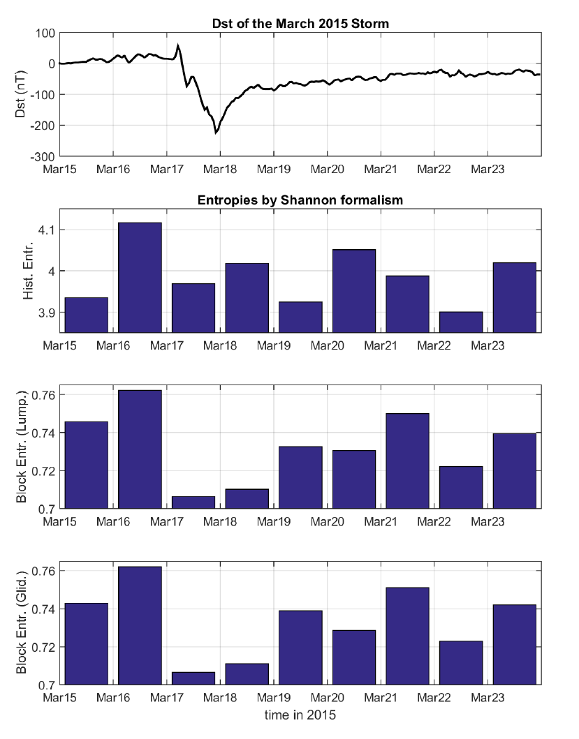
The entropy measures defined above have been computed for the case event of the 2015 St. Patrick storm (17-23 March, 2015), applying them to the time series of B_∥ , B_o1, B_o2 from Swarm A and B, and N_e for Swarm A only.

Moreover, it has been shown as Dst-like and AE-like indices can be computed from Swarm magnetic data, and a characterisation of them in terms of entropy analysis has been performed.

3. INTENS main outcomes

3.1 Ionosphere scaling features at high latitudes during geomagnetic storms

Regarding the dynamical description of the scaling features of magnetic field and electron density during the development of a typical geomagnetic storm, the most striking results come from the high-latitude regions. We looked for scaling invariance in the electron density and magnetic field fluctuations (in terms of self-similarity) supporting the idea that turbulence might play a role in generating plasma irregularities. Based on this idea we investigated a possible link between the observed scaling features and the electron density irregularities identified by RODI.

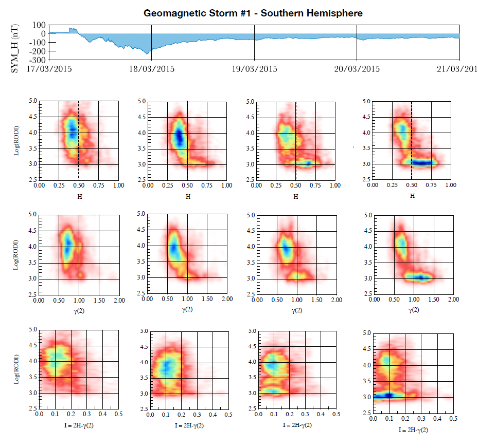
The analysis highlighted two families of plasma irregularities that seem to be associated with different physical properties. In Figure 1 we can see an example of joint probability distributions between RODI and Hurst index (first row of plots), RODI and \(\gamma(2)\) (second row of plots), RODI and I (third row of plots), for the days encompassing the maximum intensity of the 2015’s St Patrick storm (17 to 20 March 2015 from left to right), in the Southern hemisphere:

1. From one side, there are plasma density variations associated with low values of RODI that are characterized by scaling properties not supporting the idea of a fluid and/or MHD turbulence as a source of these perturbations. These irregularities mainly occur in the mid-latitude regions below the auroral oval.
2. From the other side, there are plasma density variations associated with high RODI values (> 10^3.5 cm^-3 s^-1) and scale-invariant anti-persistent fluctuations that are characterized by spectral properties similar to those expected in the case of fluid and/or MHD turbulence. Indeed, in this case, the second-order scaling exponent to which the spectral feature is related, ranges from 0.5 to 0.8, supporting a near-Kolmogorov scaling of the observed density fluctuations. These irregularities mainly occur at high latitudes in the auroral and polar cap regions and can be caused by direct particle precipitation and by dynamic plasma processes in the polar ionosphere. In other words they could be associated with a fluid/MHD plasma turbulence mechanisms generated by Kelvin-Helmholtz or shear flow instabilities.

These observations suggest that RODI, which is a proxy of ionospheric irregularities, cannot be generically considered as a proxy of the occurrence of ionospheric fluid/MHD turbulence. It is nevertheless true that its highest values (> 10^3.5 cm^-3 s^-1) can give us information on the possible turbulent origin of the plasma irregularities.

For what concerns the magnetic field fluctuations we directed our attention on the magnetic field component orthogonal to the main magnetic field, finding that the temporal evolution of the scaling properties of magnetic fluctuations during the development of each geomagnetic storm are strongly characterized by a persistent behaviour. During geomagnetically disturbed periods, the ionospheric current systems increase their intensity being the degree of ionospheric activity primarily controlled by the solar wind-magnetosphere interaction. These currents are remarkable for their strength and persistence during geomagnetically disturbed periods. The strength and persistence on time scales longer than those analyzed in our study can be responsible for the magnetic field fluctuations to cluster along a direction.

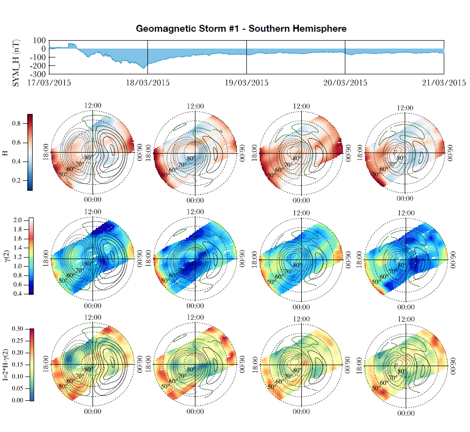
There is not a correspondence between the spatial and temporal variations of the scaling properties of the magnetic field fluctuations and the spatial and temporal variations of the mean ionospheric convection patterns. There seems to be only one match between the boundary of the auroral oval and the maximum values of intermittency, I. This correspondence is clearly visible in the Southern hemisphere where due to the greater distance between the geographic pole and the magnetic one the satellite measurements cover a wider region in the chosen coordinate system.

This correspondence is visible during the main phase and the initial of the recovery phase of each storm. The high values of intermittency seem to be able to describe the position of the auroral oval where the dynamics behaviors of the magnetic field fluctuations are characterized by singular events that are spatially localized and transient.

An example is shown in Figure 2, below, which shows the daily evolution of the Hurst index, \(\gamma(2)\), and I during the 2015’s St. Patrick storm in the Southern hemisphere, related to the magnetic field fluctuations. The SuperDARN average convection patterns inferred from the CS10 model are superimposed on the scaling maps.

All the distribution maps of scaling indices at high latitudes related to magnetic field and electron density fluctuations for the six storms studied are available in the Data Access page.

3.2 Climatology of ionospheric scaling features

The results obtained analyzing six different geomagnetic storms have been also confirmed analyzing the whole dataset (4 years from April 2014 to March 2018). Indeed, the analysis done in the project allowed producing also very interesting outcomes in terms of climatological maps of the scaling features of both magnetic field and electron density fluctuations as a function of geomagnetic activity levels and interplanetary conditions (IMF orientations).

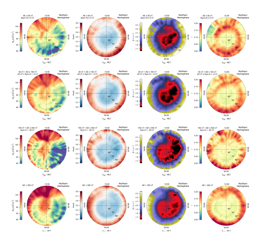
A clear dependence of the scaling features of the electron density fluctuations on both geomagnetic activity levels and interplanetary conditions have been found. In both hemispheres, at high latitudes, the electron density fluctuations are anti-persistent and characterized by spectral properties similar to those expected in the case of fluid and/or MHD turbulence. The boundary of this region seems to be the signature of plasmapause projected into the ionosphere plane. The configuration and dynamics of the plasmapause are highly sensitive to geomagnetic disturbances. During extended periods of relatively quiet geomagnetic conditions the plasmasphere expands and the plasmapause can become diffuse.

In Figure 3 one can see an example of electron density distributions, and related scaling parameters, for Swarm A, Northern hemisphere. From top to bottom the distributions are displayed as a function of the varying geomagnetic activity following the classification in sectors as explained in Section 2 above.

Conversely, during increasing magnetospheric activity, the plasmasphere gets compressed and the plasmapause is eroded forming drainage plume, whose signature on the ground is the so-called storm-enhanced density (SED) in the high and subauroral latitude ionosphere. The dynamic evolution of the plasmasphere boundary layer from quiet to disturbed period can be recognized in the dynamic evolution of the scaling features of electron density fluctuations. The ionospheric regions which are signature of the outer plasmasphere are characterized by scaling features completely different from the other regions.

All the distribution maps of scaling indices at high and mid- low-latitudes related to magnetic field and electron density fluctuations for the climatological study are available in the Data Access page.

3.3 Information entropy analysis applied to Swarm data

Finally, we have exploited the application of many novel concepts originated in dynamical systems or information theory. New methods and toolboxes for the analysis of nonlinear time series that can allow to understand the behavior of the complex solar wind-magnetosphere- ionosphere-thermosphere (MIT) coupling system and its components have been applied. In detail, we applied a series of entropy methods to the time series of the Earth's magnetic field and electron density measured by the Swarm constellation. These methods permitted us to study dynamical complexity at various scales, from a few minutes to several hours, including the investigation of the turbulent character of the topside ionosphere at both quiet and storm times.

In Figure 4 we show an example of entropy measures computed during the 2015 St. Patrick’s storm on the time series of the total magnetic field as observed by Swarm A.

The applied methods showed the complexity dissimilarity among different "physiological" (normal) and "pathological" states (intense magnetic storms) of the MIT system, implying the emergence of two distinct patterns:

1. A pattern associated with quiet periods, which is characterized by a lower degree of organization / higher complexity;
2. A pattern associated with the intense magnetic storms, which is characterized by a higher degree of organization / lower complexity.

At least, we examined the associated ionospheric response at Swarm altitudes through the derivation of a Swarm AE-like index and a Swarm Dst-like index. The newly proposed indices monitor magnetic storm activity at least as good as the standard ground-based indices. It yet remains to be investigated whether the standard AE and Dst indices or the newly proposed Swarm AE and Dst indices provide a better representation of the currents contributing to the coupled MIT system (e.g. electrojet, ring current), especially during periods of high geomagnetic activity which are of interest for prediction purposes.

In Figure 5 one can see how the Swarm-derived Dst-like index matches very well with the official Dst index for the case of 2015’s St. Patrick storm.

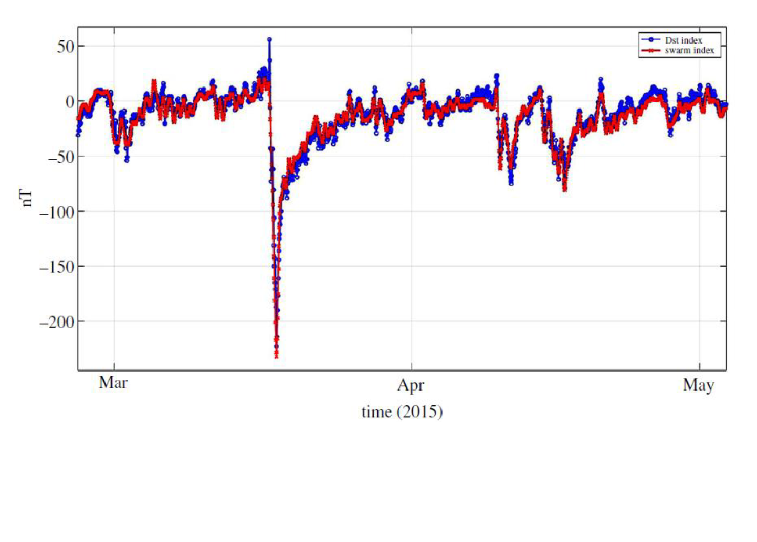
All the plots related to entropy analysis on the 2015 St. Patrick's storm and on the Swarm Dst-like index are available in the Data Access page.

Bibliography

• Cousins E. D. P., and S. G. Shepherd (2010), A dynamical model of high-latitude convection derived from SuperDARN plasma drift measurements. Journal of Geophysical Research, 115, A12329, doi:10.1029/2010JA016017.
• De Michelis P., G. Consolini, and R. Tozzi (2015), Magnetic field fluctuation features at Swarm’s altitude: A fractal approach, Geophys. Res. Lett., 42, 31003105, doi:10.1002/2015GL063603.
• Emmert A. D., D. P. Richmond, and D. P. Drob (2010), A computationally compact representation of magnetic apex and quasi dipole coordinates with smooth base vectors, J. Geophys. Res., 115, doi:10.1029/2010JA015326.
• Finlay C. C., N. Olsen, S. Kotsiaros, N. Gillet, and L. Tøffner-Clausen (2016), Recent geomagnetic secular variation from Swarm and ground observatories as estimated in the CHAOS-6 geomagnetic field model, Earth Planets and Space, 68, 112, doi: 10.1186/s40623-016-0486-1.
• Jin, Y., Spicher, A., Xiong, C., Clausen, L. B. N., Kervalishvili, G., Stolle, C., and W. J. Miloch (2019), Ionospheric plasma irregularities characterized by the Swarm satellites: Statistics at high latitudes. J. Geophys. Res. Space Physics, 124, 1262-1282.
• Kolmogorov A. (1941), The Local Structure of Turbulence in Incompressible Viscous Fluid for Very Large Reynolds’ Numbers, Doklady Akademiia Nauk SSSR, 30, 301.
• Kotsiantis S., and D. Kanellopoulos (2006), Discretization Techniques: A recent survey, GESTS International Transactions on Computer Science and Engineering, Vol. 32, 1, 47-58.
• Pincus S.M. (1991), Approximate entropy as a measure of system complexity, Proc. Natl. Acad. Sci. USA, 88, 2297-2301.
• Richman J. S., and J. R. Moorman (2000), Physiological time-series analysis using approximate and sample entropy, Am. J. Physiol. Heart Circ. Physiol., 278, 2039-2049.
• Shannon C. E. (1948), A Mathematical Theory of Communication, Bell Syst. Tech. J., 27, 379-423.
• Tsallis, C. (1988), Possible generalization of Boltzmann-Gibbs statistics, J. Stat. Phys., 52, 479-487.
• Tsallis, C. (1998), Generalized entropy-based criterion for consistent testing, Phys. Rev. E., 58, 1442-1445.